circlss among circular-response regression packages
Source:vignettes/articles/comparison.Rmd
comparison.Rmdcirclss provides capacity to fit distributional
regression for circular responses: every parameter of a
circular distribution gets its own penalized-spline predictor,
REML-selected through mgcv::gam(), across a library of
circular families.
Where circlss sits
| Package | Approach | Inference | Families | Nonlinear effects | Per-parameter | Mixtures | Geometries |
|---|---|---|---|---|---|---|---|
| circlss | mgcv penalized-spline GAMLSS | Freq. (REML/EFS) | 12 | splines (+cyclic) | every param | EM | c~l, c~c, l~c |
| circular | lm.circular |
Freq. ML | vM | linear | location | — | c~l, c~c |
| Directional | spml.reg |
Freq. ML | proj. normal | linear | location (+scale) | — | c~l, c~c |
| bpnreg | bpnr |
Bayes (MCMC) | proj. normal | linear | location (2D) | mixed eff. | c~l |
| brms | von_mises |
Bayes (Stan) | vM |
s()/t2()
|
κ | mixture() |
c~l, c~c |
| VGAM |
vgam/vglm
|
Freq. ML/IRLS | vM | vector s()
|
loc + scale | — | c~l |
| NPCirc | kernel (NW/LL) | Nonparam. | vM kernel | kernel | mean only | — | c~l, c~c, l~c |
| BAMBI | fit_angmix |
Bayes/ML | vM, wN, vmsin/cos | none | — | yes | — (density) |
# Every comparator is on CRAN:
install.packages(c("circular", "NPCirc", "bpnreg", "brms", "Directional", "VGAM", "BAMBI"))
1. c~l regression: circular response, linear
covariate
Fisher & Lee’s 31 periwinkles: direction moved (circular) on
distance moved (linear) — the shared example of circular
and NPCirc. The snails’ headings turn with distance
and tighten as they go, which splits into two
questions: the mean (§1a) and the concentration (§1b).
library(circlss); library(NPCirc); library(circular)
data(periwinkles, package = "circlss")         # Fisher & Lee's data, bundled in circlss
dist  <- periwinkles$x                          # distance moved
dir_c <- circular(periwinkles$theta.deg, units = "degrees")            # degrees, for NPCirc
peri  <- data.frame(distance = periwinkles$x, direction = periwinkles$theta.rad)
1a. The mean direction — every method agrees
circular: a von Mises link
mu = mu0 + 2*atan(b*x); location only, one global
concentration.
lm.circular(y = circular(peri$direction), x = dist, type = "c-l", init = 0)#> Circular-Linear Regression
#> Coefficients: Estimate Std. Error t value Pr(>|t|)
#> [1,] -0.008344 0.001361 6.129 4.4e-10 ***
#> Summary: (mu in radians) mu: 2.427 (0.112) kappa: 3.229 (0.717)NPCirc: a nonparametric conditional-mean curve (Nadaraya–Watson).
kern.reg.lin.circ(dist, dir_c, t = NULL, bw = 12.7, method = "NW")#> Call: kern.reg.lin.circ(x = dist, y = dir_c, bw = 12.7, method = "NW")
#> Data: dist (31 obs.); Bandwidth 'bw' = 12.7 Rho: 0.94circlss (κ ~ 1): a von Mises GAMLSS — a
penalized spline for the mean, one constant concentration. The model
circular fits, with a spline in place of the rigid atan
link.
library(circlss)
b <- circ_gam(list(direction ~ s(distance, k = 5),   # mu(distance), penalized smooth
                            ~ 1),                     # kappa constant, the fair baseline
              data = peri, family = vmlss())
summary(b)
#> Family: vmlss Link function: tanhalf log
#>
#> Parametric coefficients:
#> Estimate Std. Error z value Pr(>|z|)
#> (Intercept) 0.03544 0.05768 0.615 0.539 # mu intercept
#> (Intercept).1 1.16393 0.22185 5.246 1.6e-07 *** # log-kappa intercept -> kappa 3.20
#>
#> Approximate significance of smooth terms:
#> edf Ref.df Chi.sq p-value
#> s(distance) 1 1.001 8.7 0.00318 **
#>
#> Deviance explained = 20% -REML = 33.818 n = 31The three fixed-κ fits trace one mean curve, and the two that
estimate a concentration land on the same value: circular κ
= 3.23, circlss κ = 3.20.
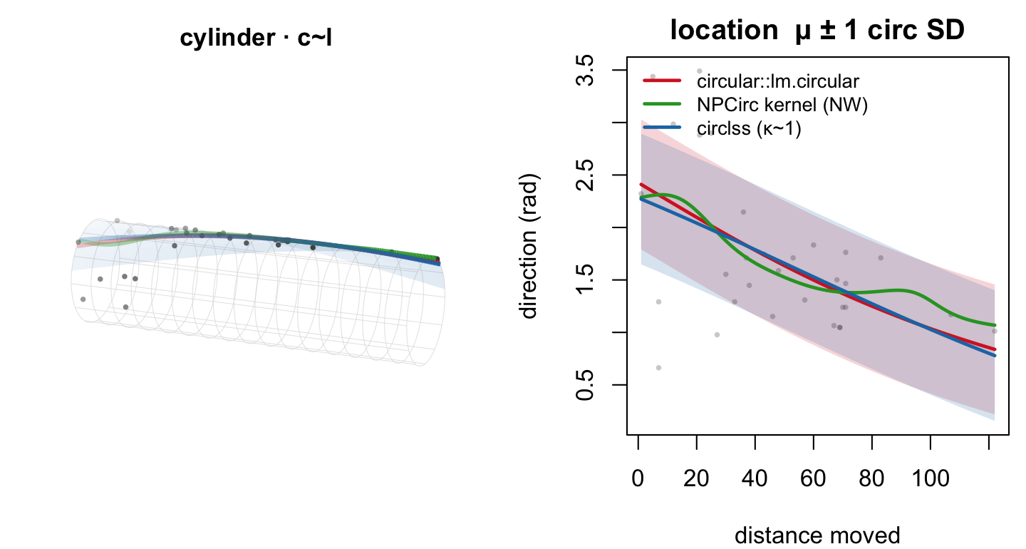
circular’s
rigid atan link, NPCirc’s Nadaraya–Watson kernel, and
circlss’s penalized spline (κ~1) trace one mean curve — headings turning
≈2.4 → 1.0 rad with distance — and the two that carry a concentration
agree on it (overlapping ±1 circ-SD bands, κ ≈ 3.2). What none of them
shows is that κ is not constant.1b. The concentration — modelling κ(distance)
The headings tighten with distance; expressing that needs a smooth on
κ, not just μ. This is where the von Mises fit turns
numerically hard — κ climbs past 150, past which the Bessel weights
I₁/I₀ overflow.
circlss puts a shrinkage smooth on log-κ:
b2 <- circ_gam(list(direction ~ s(distance, k = 5),      # mu(distance)
                             ~ s(distance, bs = "ts")),   # log-kappa smooth, SHRINKAGE basis
               data = peri, family = vmlss())
summary(b2)
predict(b2, newdata = data.frame(distance = quantile(dist, c(0, .5, 1))), type = "response")
#> Approximate significance of smooth terms:
#> edf Ref.df Chi.sq p-value
#> s(distance) 1.0001 1 21.50 4.57e-06 *** # mu smooth
#> s.1(distance) 0.9745 9 21.20 2.23e-06 *** # log-kappa smooth (ts), shrunk to edf ~1
#>
#> Deviance explained = 47.1% -REML = 27.117 n = 31
#>
#> mu kappa
#> 0% 1.974 0.790 # near-uniform heading at the shortest distance
#> 50% 1.616 5.572
#> 100% 1.024 152.219 # near-deterministic at the longestThe bs="ts" (shrinkage) basis is the whole point: its
extra null-space penalty lets REML pull the κ smooth toward flat exactly
where an unpenalized smooth would run away — here it settles on a
near-linear log climb (edf 0.97), the numerically stable shape. That
shrinkage is what keeps the fit inside the safe region.
VGAM is the natural frequentist peer — its
vonmises() family carries its own predictor for
both the location and the concentration.
library(VGAM)
peri$dir02 <- peri$direction %% (2 * pi)                 # vonmises support is (0, 2pi)
vgam(dir02 ~ s(distance), vonmises, data = peri)         # smooth on BOTH parameters
vglm(dir02 ~ distance,    vonmises, data = peri)         # linear location + linear log-kappa
#> vgam(dir02 ~ s(distance), vonmises):
#> Error: NAs in the working weights var 'wz' # the smooth-kappa IRLS overflows
#>
#> vglm(dir02 ~ distance, vonmises): [converges; :1 = location, :2 = log-kappa]
#> Estimate Std. Error z value Pr(>|z|)
#> (Intercept):1 -0.702598 0.139260 -5.045 4.5e-07 *** # location (extended-logit link)
#> (Intercept):2 -0.344285 0.504981 -0.682 0.495 # log-kappa intercept
#> distance:1 -0.007602 0.001545 -4.921 8.6e-07 ***
#> distance:2 0.044872 0.009077 4.944 7.7e-07 *** # log-kappa slope == circlss's 0.045
#> Names of linear predictors: extlogitlink(location), loglink(scale)
#> fitted kappa: 0.74 (nearest snail) -> 169.0 (farthest)VGAM’s smooth-on-both vgam() hits the same wall — its
IRLS working weights overflow. The linear vglm() converges,
its log-κ slope (0.045) matches circlss’s, and its fitted κ climbs 0.7 →
169, landing right on circlss’s smooth.
brms offers a Bayesian smooth on κ, but the natural
kappa ~ s(distance) (or kappa ~ distance)
overflows Stan on these 31 points — κ = exp(η) runs to infinity during
sampling.
library(brms)
pb <- transform(peri, direction = atan2(sin(direction), cos(direction)))   # (-pi, pi]
brm(bf(direction ~ s(distance), kappa ~ distance), data = pb, family = von_mises())
#> Error: Exception: boost::math::cyl_bessel_i<double>: numeric overflow
brm(bf(direction ~ s(distance), kappa ~ 1), data = pb, family = von_mises(),   # held at kappa~1
    chains = 2, iter = 1000, seed = 1)
#> Estimate Est.Error Q2.5 Q97.5
#> Intercept 1.303 0.198 0.991 1.752
#> kappa_Intercept 1.089 0.211 0.668 1.475 # kappa ~ 3.0, constant
#> sdistance_1 -1.738 2.213 -6.543 3.303The overflow is a reparametrization artefact, not a dead end:
standardize the covariate (kappa ~ scale(distance)) and
tighten the κ prior, and the crash disappears — brms then recovers the
same climb (κ → ≈160, agreeing with circlss and VGAM). But the posterior
for a concentration that spans two orders of magnitude on 31 points is
funnel-shaped, and the sampler still throws hundreds of divergent
transitions (here 526 of 6000 draws) that pushing
adapt_delta to 0.999 does not clear. Only circlss fits the
smooth κ directly and cleanly — a ts-penalized
REML optimization, no sampler to diverge, no covariate surgery — which
is why it alone is drawn as an honest smooth.
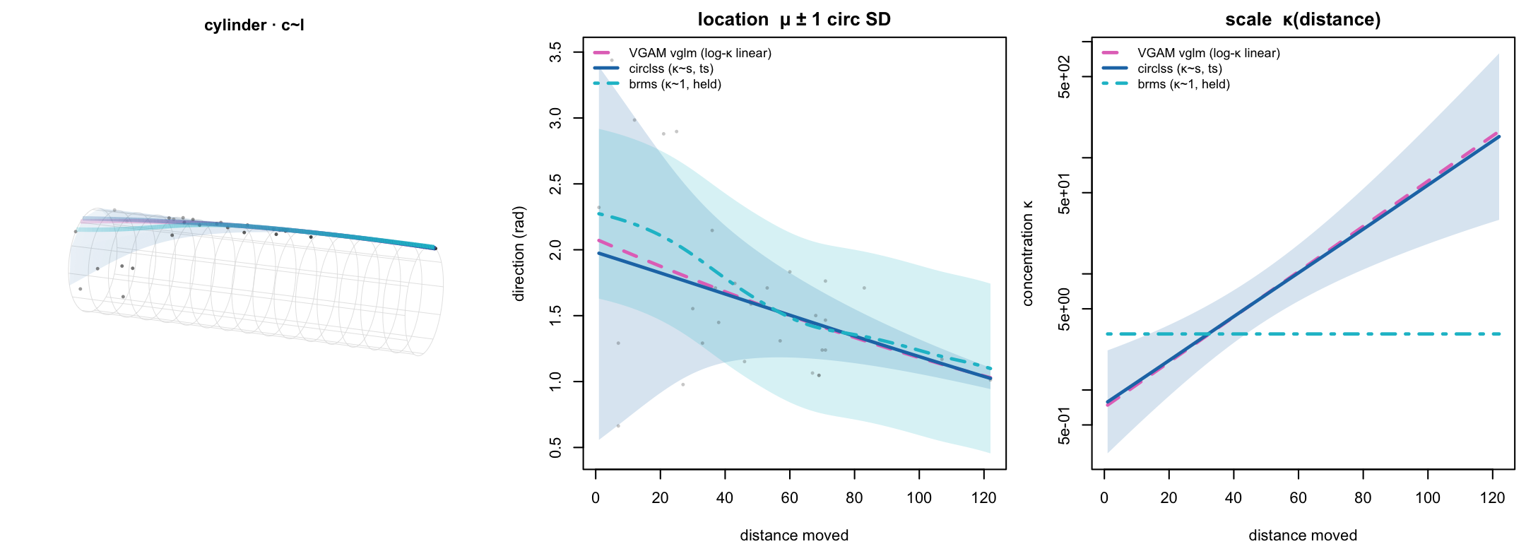
bs="ts" smooth
climbs κ 0.8 → 152 with a 2-SE band, and VGAM’s linear-log-κ
vglm (κ 0.7 → 169) lands on top of it — the ±1 circ-SD band
(centre) pinching shut as the headings tighten. brms is held flat at
κ~1: its kappa ~ s(distance) overflows Stan’s Bessel
evaluation; VGAM’s smooth-on-both vgam() overflows too.
Only circlss draws the smooth κ(distance), because the ts
shrinkage penalty holds it in the numerically stable region.2. One distribution, three inference engines — projected normal
bpnreg’s Motor data: 42 hand-movement phases under three
priming conditions. The projected normal writes an angle as
atan2(mu2, mu1) of two linear predictors, the same form
bpnr (Gibbs), spml.reg (ML), and circlss
pnlss (REML) all fit.
fit_b <- bpnr(Phaserad ~ Cond + AvAmp, data = Motor, its = 5000, burn = 1000, seed = 1)
round(coef_lin(fit_b)[, c("mean", "sd")], 3)                  # bpnreg, Gibbs

X <- model.matrix(~ Cond + AvAmp, Motor)[, -1]
spml.reg(Motor$Phaserad, X, rads = TRUE)$be                  # Directional, ML

b <- circ_gam(list(Phaserad ~ Cond + AvAmp, ~ Cond + AvAmp),  # circlss pnlss, REML
              data = Motor, family = pnlss())
summary(b)
#> bpnreg coef_lin (component I rows 1-4, II rows 5-8) Directional $be
#> mean sd cos(y) sin(y)
#> (Intercept) 1.337 0.452 (Intercept) 1.338 1.401
#> Condsemi.imp -0.476 0.637 Condsemi.imp -0.382 -1.126
#> Condimp -0.605 0.656 Condimp -0.522 -0.907
#> AvAmp -0.010 0.012 AvAmp -0.009 -0.011
#> ... # circlss pnlss summary:
#> (Intercept).1 1.397 0.438 (Intercept).1 1.39719 z = 3.192 0.0014 **
#> Condsemi.imp.1 -1.162 ... Condsemi.imp.1 -1.16182 z = -1.953 0.051 .
#> Deviance explained = 12.9% -REML = 65.46 n = 42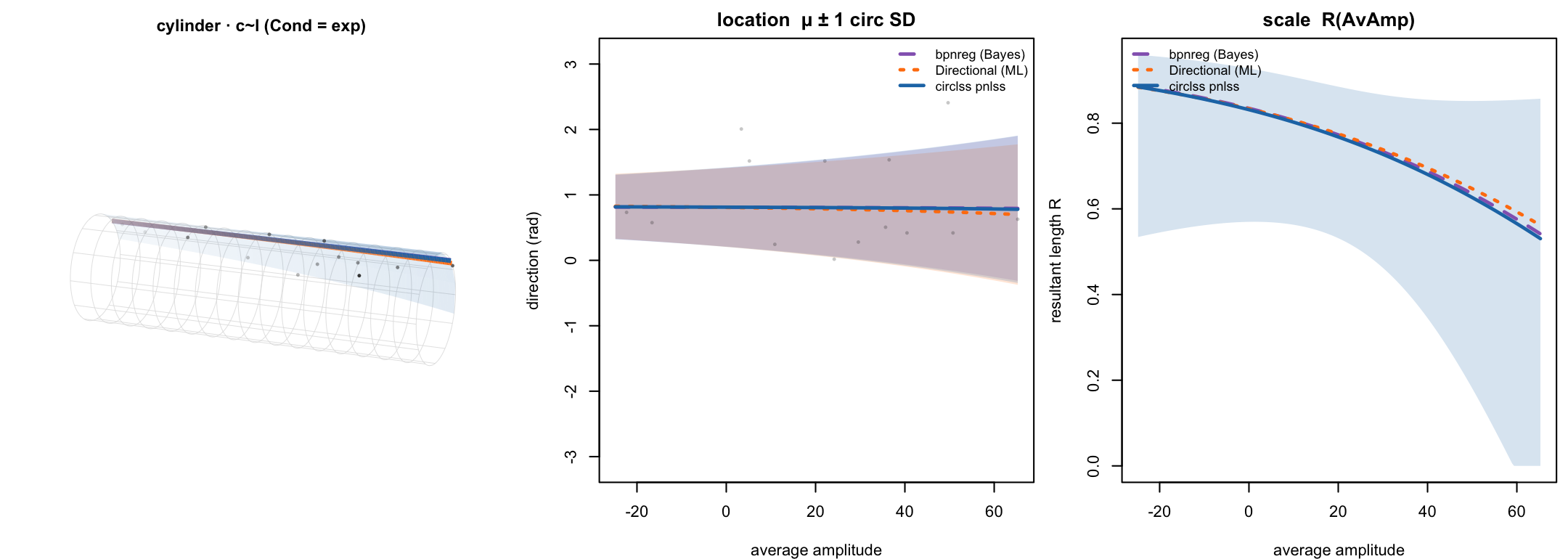
Cond + AvAmp could become Cond + s(AvAmp) — a
smooth neither neighbour offers.3. c~c circular-circular regression
wind direction, 6 a.m. to noon
data(wind)
i6 <- seq(7, 1752, by = 24); i12 <- seq(13, 1752, by = 24)   # daily 06:00, 12:00
wr <- function(a) atan2(sin(a), cos(a))
dcc <- data.frame(w6 = wr(wind$wind.dir[i6]), w12 = wr(wind$wind.dir[i12]))

kern.reg.circ.circ(circular(dcc$w6), circular(dcc$w12), bw = 6.1, method = "NW")
# winding response -> projected normal (a von Mises mean can't follow a heading
# that goes round the circle); mean AND concentration each a cyclic smooth:
b_cc <- circ_gam(list(w12 ~ s(w6, bs = "cc"), ~ s(w6, bs = "cc")),
                 data = dcc, family = pnlss())
summary(b_cc)$s.table
#> Family: pnlss n = 73 Deviance explained = 46%
#> edf Ref.df Chi.sq p-value
#> s(w6) 2.894 8 33.66 <2e-16 *** # mean direction smooth
#> s.1(w6) 2.974 8 31.04 <2e-16 *** # concentration smooth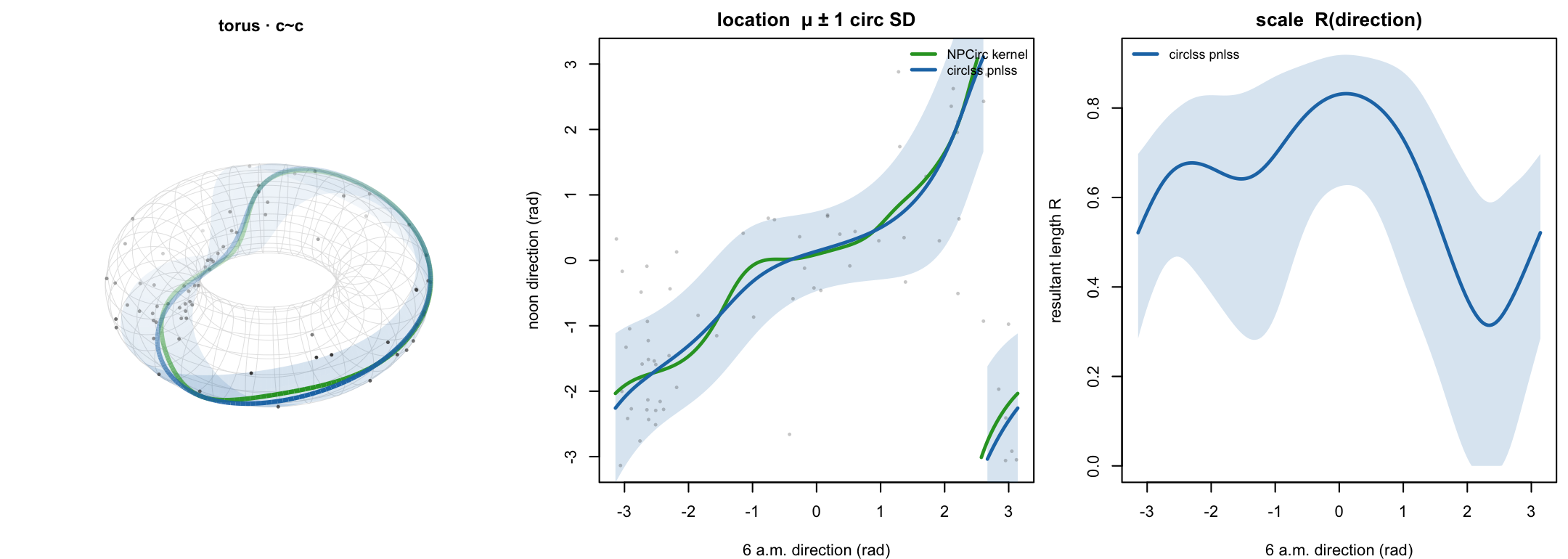
pnlss fits the
mean (edf 2.9) and the concentration (edf 3.0), both
p < 2×10⁻¹⁶ — the varying spread (right) is the part the
kernel has no parameter for.4. l~c linear-circular regression
does wind speed depend on direction?
data(speed.wind2)
sw <- na.omit(data.frame(dir = speed.wind2$Direction, speed = speed.wind2$Speed))
sw$rad <- wr(sw$dir * pi / 180)

kern.reg.circ.lin(circular(sw$dir, units = "degrees"), sw$speed, method = "LL")
# model BOTH the mean and the SD (gausslss, tau = 1/sigma) of speed by direction:
b_lc  <- circ_gam(list(speed ~ s(rad, bs = "cc"), ~ s(rad, bs = "cc")),
                  data = sw, family = gausslss())
# mean alone under GCV (the less-conservative selector a kernel resembles):
b_gcv <- circ_gam(speed ~ s(rad, bs = "cc"), family = gaussian(), method = "GCV.Cp", data = sw)
summary(b_lc)$s.table; summary(b_gcv)$s.table
#> gausslss edf Ref.df Chi.sq p-value
#> s(rad) [mean] 0.001 8 0.001 0.465 # mean: flat under REML
#> s.1(rad) [SD] 2.016 8 8.027 0.009 # SD: varies with direction
#> gaussian (GCV) edf Ref.df F p-value
#> s(rad) [mean] 6.436 8 1.815 0.028 # mean: wiggly under GCV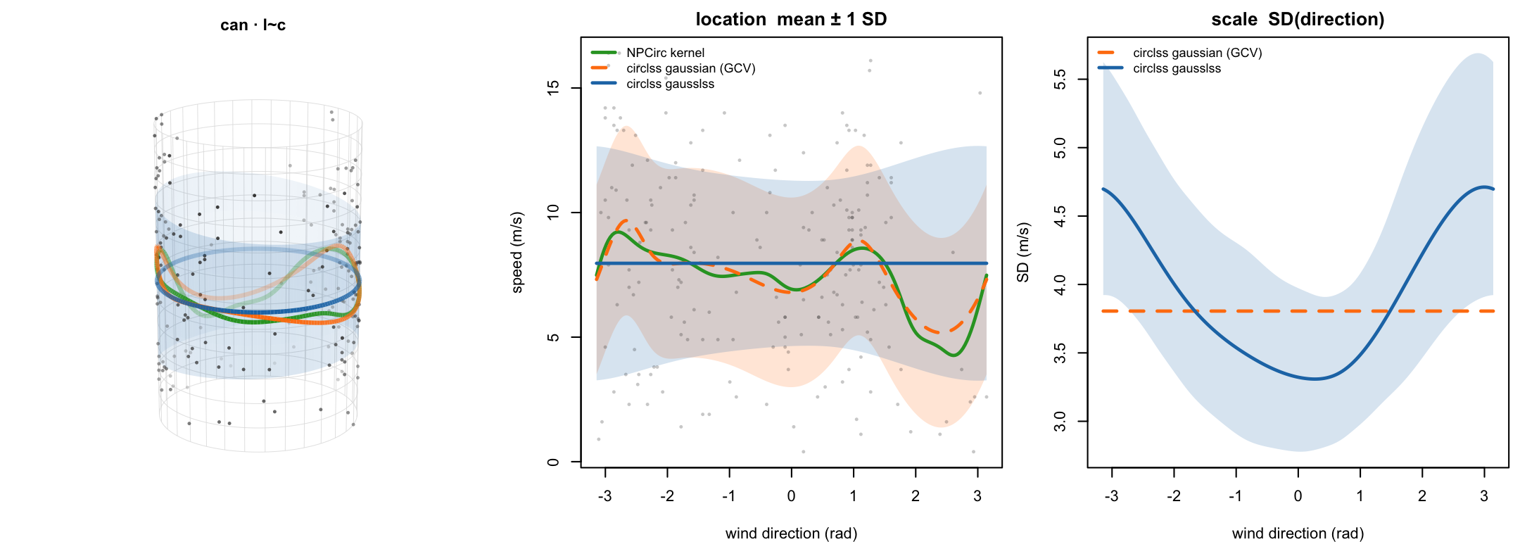
5. Mixtures — BAMBI vs circ_mix
Not a regression: BAMBI fits fixed-form mixtures of
toroidal densities. For the 8TIM protein’s 490 (φ, ψ) backbone
dihedrals, a four-component bivariate sine von Mises captures the
Ramachandran basins. circ_mix reaches the same clusters by
EM over circular GAMs, each component a conditional f(ψ | φ) × marginal
f(φ).
library(BAMBI); data(tim8)
fit_angmix("vmsin", tim8, ncomp = 4, n.iter = 500, n.chains = 1)        # BAMBI, HMC

circ_mix(list(psi ~ cos(phi) + sin(phi), phi ~ 1),                      # circ_mix, EM
         data = tim8, family = vmlss(), K = 4)
#> BAMBI: 4 component vmsin mixture, 490 obs, fitted via HMC.
#>
#> Finite mixture of circular GAMs (circ_mix) -- joint torus density
#> family vmlss | K = 4 components | 490 obs BIC = 1751.77
#> components (MAP): pi = 0.293 / 0.474 / 0.200 / 0.032 (n = 152 / 236 / 86 / 16)
#> converged in 95 iterations; restart basin hits 1/10.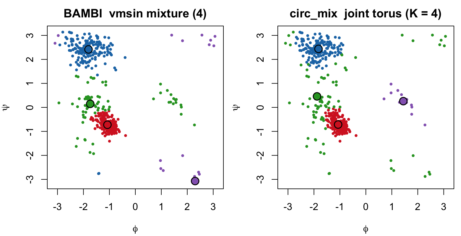
BAMBI is Bayesian and covariate-free; circ_mix
is built on circ_gam, so the components that here cluster a
static density can instead carry the smooths and covariates of
§1–3.